1. Data Exploration & Pre-Processing
Before we begin building a recommender system we must first get a sense of the dataset. The objective of this chapter is to explore the dataset and to perform any necessary pre-processing of the data. We will use pandas to read in and explore the data. We will sanity check the data, handle inconsistencies and outliers, and make sure the data can be used to build an accurate and reliable recommender system.
1.1. Imports
import pandas as pd
import numpy as np
import matplotlib.pyplot as plt
import seaborn as sns
from sklearn import preprocessing
1.2. Read in Data
artists = pd.read_csv('..\\data\\hetrec2011-lastfm-2k\\artists.dat', sep='\t', encoding='latin-1')
tags = pd.read_csv('..\\data\\hetrec2011-lastfm-2k\\tags.dat', sep='\t', encoding='latin-1')
user_artists = pd.read_csv('..\\data\\hetrec2011-lastfm-2k\\user_artists.dat', sep='\t', encoding='latin-1')
user_friends = pd.read_csv('..\\data\\hetrec2011-lastfm-2k\\user_friends.dat', sep='\t', encoding='latin-1')
user_tagged_artists = pd.read_csv('..\\data\\hetrec2011-lastfm-2k\\user_taggedartists.dat', sep='\t', encoding='latin-1')
1.3. Overview of the DataFrames
1.3.1. artists
This dataframe contains information about 17,632 music artists listened to and tagged by the users.
artists.head(3)
| id | name | url | pictureURL | |
|---|---|---|---|---|
| 0 | 1 | MALICE MIZER | http://www.last.fm/music/MALICE+MIZER | http://userserve-ak.last.fm/serve/252/10808.jpg |
| 1 | 2 | Diary of Dreams | http://www.last.fm/music/Diary+of+Dreams | http://userserve-ak.last.fm/serve/252/3052066.jpg |
| 2 | 3 | Carpathian Forest | http://www.last.fm/music/Carpathian+Forest | http://userserve-ak.last.fm/serve/252/40222717... |
print('number of rows: ' + str(artists.shape[0]))
pd.DataFrame([artists.nunique(),artists.isna().sum()], index=['unique_entries','null_values']).T
number of rows: 17632
| unique_entries | null_values | |
|---|---|---|
| id | 17632 | 0 |
| name | 17632 | 0 |
| url | 17632 | 0 |
| pictureURL | 17188 | 444 |
Delete pcitureURL column
The column pcitureURL contains links that cannot be accessed, and has no use to us, so we will delete it.
del artists['pictureURL']
Reset ids
Set id to start from 0 and to be consecutive.
artist_id_dict = pd.Series(artists.index.values,index=artists.id).to_dict()
artists.id = artists.id.map(artist_id_dict)
print('number of rows: ' + str(artists.shape[0]))
pd.DataFrame([artists.nunique(),artists.isna().sum()], index=['unique_entries','null_values']).T
number of rows: 17632
| unique_entries | null_values | |
|---|---|---|
| id | 17632 | 0 |
| name | 17632 | 0 |
| url | 17632 | 0 |
1.3.2. tags
This dataframe contains the set of all tags available in the dataset. Tags can be informative of the musical genre.
tags.head(3)
| tagID | tagValue | |
|---|---|---|
| 0 | 1 | metal |
| 1 | 2 | alternative metal |
| 2 | 3 | goth rock |
print('number of rows: ' + str(tags.shape[0]))
pd.DataFrame([tags.nunique(),tags.isna().sum()], index=['unique_entries','null_values']).T
number of rows: 11946
| unique_entries | null_values | |
|---|---|---|
| tagID | 11946 | 0 |
| tagValue | 11946 | 0 |
Reset ids
Similar to artist id, reset tagID to start from 0 and to be consecutive.
tags_dict = pd.Series(tags.index.values,index=tags.tagID).to_dict()
tags.tagID = tags.tagID.map(tags_dict)
1.3.3. user_artists
The dataframe contains the artists listened to by each user, as well as a listening count (weight) for each user, artist pair.
user_artists.head()
| userID | artistID | weight | |
|---|---|---|---|
| 0 | 2 | 51 | 13883 |
| 1 | 2 | 52 | 11690 |
| 2 | 2 | 53 | 11351 |
| 3 | 2 | 54 | 10300 |
| 4 | 2 | 55 | 8983 |
print('number of rows: ' + str(user_artists.shape[0]))
pd.DataFrame([user_artists.nunique(),user_artists.isna().sum()], index=['unique_entries','null_values']).T
number of rows: 92834
| unique_entries | null_values | |
|---|---|---|
| userID | 1892 | 0 |
| artistID | 17632 | 0 |
| weight | 5436 | 0 |
Reset userID and Map artistID
Reset userID to start from 0 and to be consecutive.
Replace artistIDs with the corresponding ids in artists.
user_id_dict = pd.Series(range(0,user_artists.userID.nunique()),index=user_artists.userID.unique()).to_dict()
user_artists.userID = user_artists.userID.map(user_id_dict)

user_artists.artistID = user_artists.artistID.map(artist_id_dict)
1.3.4. user_friends
This dataframe contains the friend relations between users in the dataset.
user_friends.head(3)
| userID | friendID | |
|---|---|---|
| 0 | 2 | 275 |
| 1 | 2 | 428 |
| 2 | 2 | 515 |
print('number of rows: ' + str(user_friends.shape[0]))
pd.DataFrame([user_friends.nunique(),user_friends.isna().sum()], index=['unique_entries','null_values']).T
number of rows: 25434
| unique_entries | null_values | |
|---|---|---|
| userID | 1892 | 0 |
| friendID | 1892 | 0 |
While the dataframe consists of 25,434 rows, it in fact only contains half this amount (12,717) of bi-directional relations, each relation is included twice, an example of which can be seen in the next cell’s output.
user_friends[((user_friends['userID'] == 2) & (user_friends['friendID'] == 275)) | ((user_friends['userID'] == 275) & (user_friends['friendID'] == 2))]
| userID | friendID | |
|---|---|---|
| 0 | 2 | 275 |
| 3837 | 275 | 2 |
Map userID and friendID
Replace both userID and friendID so they corresponding with the intended users.
user_friends.userID = user_friends.userID.map(user_id_dict)
user_friends.friendID = user_friends.friendID.map(user_id_dict)
1.3.5. user_tagged_artists
This dataframe contains the tag assignments of artists provided by each user and the accompanying date of when the tag assignments were done.
user_tagged_artists.head(3)
| userID | artistID | tagID | day | month | year | |
|---|---|---|---|---|---|---|
| 0 | 2 | 52 | 13 | 1 | 4 | 2009 |
| 1 | 2 | 52 | 15 | 1 | 4 | 2009 |
| 2 | 2 | 52 | 18 | 1 | 4 | 2009 |
print('number of rows: ' + str(user_tagged_artists.shape[0]))
pd.DataFrame([user_tagged_artists.nunique(),user_tagged_artists.isna().sum()], index=['unique_entries','null_values']).T
number of rows: 186479
| unique_entries | null_values | |
|---|---|---|
| userID | 1892 | 0 |
| artistID | 12523 | 0 |
| tagID | 9749 | 0 |
| day | 4 | 0 |
| month | 12 | 0 |
| year | 10 | 0 |
Interestingly each user has tagged at least one artist but not all artists have received a tag. The number of unique entries for the day and year seems odd and will be further investigated in the next two cells.
user_tagged_artists.day.value_counts()
1    182948
5      1505
6      1469
9       557
Name: day, dtype: int64
Considering the size of the dataframe it is inprobable that users only ever tagged on the same four days of every month, and is instead likely indicative of the days when the data was collected. Therefore, we will not place any significance on the day in further analysis.
user_tagged_artists.year.value_counts()
2010    54998
2009    43366
2008    40273
2007    20415
2011    15125
2006     9814
2005     2483
1956        3
1957        1
1979        1
Name: year, dtype: int64
Last.fm was founded in 2002, and the internet in 1983! Therefore, the 4 dates that correspond to the years 1956, 1957, or 1979 are obvious errors. The dataset was compiled in 2011 so it is conceivable that the data collected was created sometime between 2005 and 2011.
Replace years before 2005
Replace any year before 2005 with 2005
user_tagged_artists.loc[user_tagged_artists['year'] < 2005,'year'] = 2005
Map userID, artistID and tagID
user_tagged_artists.userID = user_tagged_artists.userID.map(user_id_dict)
user_tagged_artists.artistID = user_tagged_artists.artistID.map(artist_id_dict)
user_tagged_artists.tagID = user_tagged_artists.tagID.map(tags_dict)
1.4. Data Exploration & Visualisations
1.4.1. Number of artists listened to by each user
user_artists_count = pd.DataFrame([artists_df.shape[0] for user, artists_df in user_artists.groupby('userID')]).value_counts().rename_axis('number_of_artists').reset_index(name='counts')
plt.figure(figsize=(15,6))
ax = sns.histplot(data=user_artists_count,x='number_of_artists',weights='counts',bins=5)
ax.bar_label(ax.containers[0],c='r')
ax.set(title='Number of Artists Listened to by Users')
plt.show()
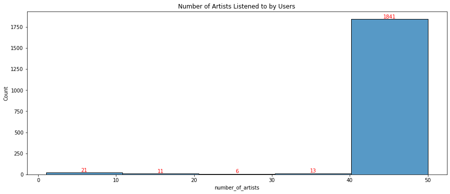
This plot is left skewed, with the vast majority of users having listened to 40-50 unique artists. Only 51 users, or 2.7% of users, have listened to fewer than 40 artists. This is reassuring as we are planning to use this dataset to build a recommender system. The more artists listened to by each user the better the recommender system should perform as the system will be better able to determine users’ musical interests and tastes.
1.4.2. Number of listeners per artist
listeners_count = user_artists.groupby('artistID').size().reset_index(name='number_of_listeners')
plt.figure(figsize=(15,6))
ax = sns.histplot(data=listeners_count,x='number_of_listeners',bins=10)
ax.bar_label(ax.containers[0],c='r')
ax.set(title='Number of Listeners per Artist')
plt.show()
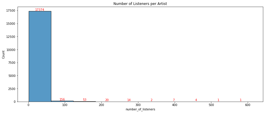
listeners_count.number_of_listeners.describe()
count    17632.000000
mean         5.265086
std         20.620315
min          1.000000
25%          1.000000
50%          1.000000
75%          3.000000
max        611.000000
Name: number_of_listeners, dtype: float64
This right skewed plot is not ideal. It is common practice for recommender systems to disgard items (in this case artists) with few iterations. However, 50% of artists in this dataset have only been listened to by a single user. If we were to exclude artists with less than a certain number of interactions we lose the majority of the dataset so we will work with what we have.
1.4.3. Weight for each user/artist pair
user_artists.weight.describe()
count     92834.00000
mean        745.24393
std        3751.32208
min           1.00000
25%         107.00000
50%         260.00000
75%         614.00000
max      352698.00000
Name: weight, dtype: float64
sns.set_style('darkgrid')
sns.boxplot(x =user_artists.weight)
plt.show()
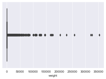
The distribution is extremely left skewed. 75% of weights are less than 614, yet the max weight is 352,698. There are extreme outliers. We believe the dataset contains data from 2005-2011. For a user to have listened to a certain artist 352,698 times over that peroiod they would have had to listen to that artist roughly 1,600 times every day. It is unlikey that these extreme outliers are extreme music lovers and is instead more conceivable that there are errors in the data.
1.4.3.1. Determine cut-off for allowable weight values
To determine the maximum weight allowed, we will group users by weight bin (0-500, 500-1000, 1000-1500 …). The logic we will apply will assume that if you have listened to one artist betweeen 500-1000 times then you’ve probably listened to other artists between 0-500 times. If you are a big music listener and have listened to your absolute favourite artist 2000+ times, then you have probably listened to another of your favourite artists between 1500-2000 times.
We will calculate the percentage of users in each bin which were also in the previous bin. E.g. what percentage of users who have at least one weight between 3000 and 3500, also have at least one weight between 2500 and 3000?
pc_users_in_both = []
incrs = list(range(50,len(user_artists.weight),500))
users_below = set()
for inc in incrs:
    users_in_inc = set(user_artists[(user_artists.weight > inc) & (user_artists.weight < (inc + 500))].userID)
    users_in_both = users_below.intersection(users_in_inc)
    if len(users_below) > 0:
        pc_users = len(users_in_both) / len(users_below) * 100
        pc_users_in_both.append(pc_users)
    else:
        pc_users_in_both.append(0)
    users_below = users_in_inc
sns.set_style('darkgrid')
sns.set(font_scale = 1)
fig, ax = plt.subplots(nrows=1, ncols=2, figsize=(12, 4))
sns.lineplot(x=incrs, y=pc_users_in_both, ax=ax[0]).set_title('% of users in bin also in lower bin')
ax[0].set(xlabel='start of bin', ylabel='percentage of users also in directly lower bin',xlim=[500,80000])
sns.lineplot(x=incrs, y=pc_users_in_both, ax=ax[1]).set_title('% of users in bin also in lower bin (zoomed in)')
ax[1].set(xlabel='start of bin', ylabel='percentage of users also in directly lower bin',xlim=[500,10000])
plt.show()
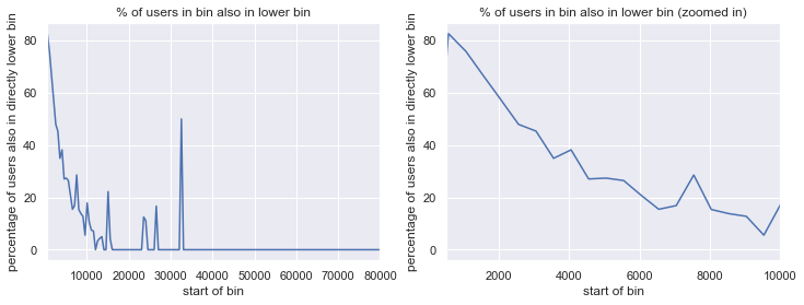
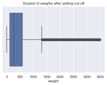
As expected the percentage of users in a bin and in the consecutive bin initially steadily decreases, as most users reach their max weight. However, the plot quick starts to fluctuate. To decide on the max allowable weight, we will focus on the right zoomed in graph. Up utill around 3,500 the graph is almost linear. Therefore, we will set the max allowable weight to the 3,500. It is possible that we will lose some super fans through this process but it is better than having errors in the data. For all weights above 3,500 we will set them to the user’s median weight if it is below 3,500, otherwise it will be set to the median weight of all users’ weights.
users_to_be_updated = user_artists.userID[user_artists['weight'] > 3500].unique()
users_artists_below_thres = user_artists[user_artists['weight'] < 3500]
user_new_weights_dict = round(users_artists_below_thres[users_artists_below_thres.userID.isin(list(users_to_be_updated))].groupby('userID').weight.median()).to_dict()
for index, row in user_artists.iterrows():
    if row.weight > 3500:
        try:
            row.weight = user_new_weights_dict[row.userID]
        except:
            artist_median = user_artists[user_artists['artistID'] == row.artistID].weight.median()
            if artist_median < 3500:
                row.weight = user_artists[user_artists['artistID'] == row.artistID].weight.median()
            else:
                row.weight = user_artists.weight.median()
sns.boxplot(x=user_artists.weight).set_title('Boxplot of weights after setting cut-off')
plt.show()
1.4.3.2. Scale the weights between 1-5
min_weight = min(user_artists.weight)
max_weight = max(user_artists.weight)
for i in range(0,len(user_artists)):
    user_artists.weight.iloc[i] = np.interp(user_artists.weight.iloc[i],[min_weight,max_weight],[1,5])
user_artists.describe()
| userID | artistID | weight | |
|---|---|---|---|
| count | 92834.000000 | 92834.000000 | 92834.000000 |
| mean | 944.222483 | 3235.736724 | 1.536476 |
| std | 546.751074 | 4197.216910 | 0.664117 |
| min | 0.000000 | 0.000000 | 1.000000 |
| 25% | 470.000000 | 430.000000 | 1.120034 |
| 50% | 944.000000 | 1237.000000 | 1.291512 |
| 75% | 1416.000000 | 4266.000000 | 1.667619 |
| max | 1891.000000 | 17631.000000 | 5.000000 |
1.4.4. Most popular artists
To find the most popular artists we will use two approaches. The first will sum all listens per artist and the second will perform a count of unique listeners per artist.
artist_pop = pd.concat([pd.DataFrame(user_artists.groupby('artistID').size()), pd.DataFrame(user_artists.groupby('artistID').weight.sum())],axis=1).set_axis(['listeners', 'listens'], axis=1, inplace=False).reset_index()
artist_pop = pd.merge(artist_pop, artists.iloc[:, 0:2], left_on='artistID', right_on='id')
bylistens = artist_pop.sort_values('listens', ascending=False).head(10)
bylisteners = artist_pop.sort_values('listeners', ascending=False).head(10)
fig, ax = plt.subplots(nrows=1, ncols=2, figsize=(12, 4))
fig.tight_layout()
sns.barplot(x=bylistens.listens, y=bylistens.name,palette="crest_r",ax=ax[0])
ax[0].set(xlabel='listens', ylabel='artist', title='most popular artists by number of LISTENS')
ax = sns.barplot(x=bylisteners.listeners, y=bylisteners.name,palette="rocket",ax=ax[1])
ax.set(xlabel='listeners', ylabel='artist', title='most popular artists by number of LISTENERS')
plt.subplots_adjust(wspace = 0.5)
plt.show()
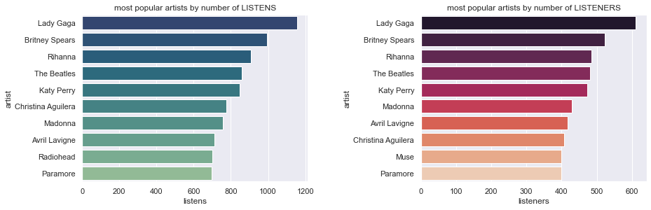
Lady Gaga appears as the top artist in both, this is reflective of listening tastes for the time period that the data was collected. While there are some differences between the two charts, on the whole popular artists have the most listens and listeners.
1.4.5. Most popular tags
Remove special characters
Special characters are causing almost identical tags to be counted as two different tags. This is an issue for tags such as 80’s and 80s. To combat this we will remove all special characters.
tag_dict = pd.Series(tags.tagValue,index=tags.tagID).to_dict()
user_tagged_artists_tag = user_tagged_artists.copy()
user_tagged_artists_tag['tag'] = user_tagged_artists_tag.tagID.map(tag_dict)
user_tagged_artists_tag.tag = user_tagged_artists_tag.tag.apply(lambda x: ''.join(char for char in x if char.isalnum()))
Group on tag
tags_ranked = user_tagged_artists_tag.groupby('tag').size().reset_index(name='counts').sort_values('counts',ascending=False)
ax = sns.barplot(x=tags_ranked.head(10).counts, y=tags_ranked.head(10).tag,palette="Greens_r")
ax.set(xlabel='count of tag usage', ylabel='tag',title='most used tags')
plt.show()
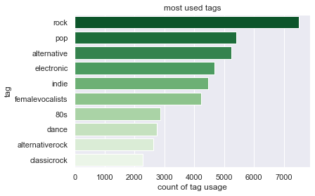
No big surprises here.
1.4.6. Can tags be used as genres?
From looking at the top tags it appears that they could be used as item features representing artist genres. I want to determine how common the top 20 tags are. For each artist tagged, I will check if at least one of their tags is also in the top 20 overall tags.
top20tags = set(tags_ranked.head(20).tag.values)
# artist_tag = user_tagged_artists.copy()
# artist_tag['tagValue'] = artist_tag.tagID.map(tag_dict)
artist_tagSet = user_tagged_artists_tag.groupby('artistID').tag.agg(lambda x:set(x.unique())).reset_index(name='tagSet')
artists_with_top_tag = 0
for index,row in artist_tagSet.iterrows():
    inters = top20tags.intersection(row.tagSet)
    if len(inters) > 0:
        artists_with_top_tag += 1
pc_artists = round(artists_with_top_tag/artist_tagSet.shape[0] * 100)
print('Percentage of tagged artists with a tag in top 20 tags: ' + str(pc_artists) + '%')
Percentage of tagged artists with a tag in top 20 tags: 63%
We can make an assumption about the primary genre of 63% of tagged artists using this approach. However, as not all artist are tagged, this would actually only cover approximately 46% of all artists. Nevertheless, there are too many unique tags to one-hot-encode all of the tags, so we will procede with the top 20 tags.
Approach:
compute set of 20 most used tags: top20tags (done)
For each artist:
Collect set of all tags: artist_tagSet
Find intersection of artist_tagSet and top20tags
If no mutual tags, leave artist tag as no_tag
Else if only one mutual tag, set artist tag as mutual tag
Else, from the set of mutual tags, find the most tag for that artist
top20tags
{'80s',
 '90s',
 'alternative',
 'alternativerock',
 'ambient',
 'british',
 'classicrock',
 'dance',
 'electronic',
 'experimental',
 'femalevocalists',
 'hardrock',
 'hiphop',
 'indie',
 'indierock',
 'metal',
 'newwave',
 'pop',
 'rock',
 'singersongwriter'}
tag_list = pd.Series(['no_tag'] * artist_tagSet.shape[0])
for index,row in artist_tagSet.iterrows():
    inters = top20tags.intersection(row.tagSet)
    if len(inters) == 1:
        tag_list[index] = str(''.join(inters))
    elif len(inters) > 1:
        tag_list[index] = user_tagged_artists_tag[user_tagged_artists_tag.artistID == row.artistID][user_tagged_artists_tag.tag.isin(inters)].groupby('tag').tag.count().reset_index(name='counts').sort_values('counts',ascending=False).tag[0]
artist_tagSet['tag'] = tag_list
C:\Users\User\AppData\Local\Temp/ipykernel_3016/3829306717.py:7: UserWarning: Boolean Series key will be reindexed to match DataFrame index.
  tag_list[index] = user_tagged_artists_tag[user_tagged_artists_tag.artistID == row.artistID][user_tagged_artists_tag.tag.isin(inters)].groupby('tag').tag.count().reset_index(name='counts').sort_values('counts',ascending=False).tag[0]
artist_tagSet.head(3)
| artistID | tagSet | tag | |
|---|---|---|---|
| 0 | 0.0 | {weeabo, jrock, japanese, gothic, betterthanla... | no_tag |
| 1 | 1.0 | {truegothemo, seenlive, german, gothicrock, vo... | ambient |
| 2 | 2.0 | {blackmetal, norwegianblackmetal, saxophones, ... | no_tag |
One-Hot Encoding
genres = pd.get_dummies(artist_tagSet['tag'])
artist_features = pd.concat([artists, genres], axis=1).fillna(0)
del artist_features['url']
artist_features.head(3)
| id | name | 80s | 90s | alternative | alternativerock | ambient | british | classicrock | dance | ... | hardrock | hiphop | indie | indierock | metal | newwave | no_tag | pop | rock | singersongwriter | |
|---|---|---|---|---|---|---|---|---|---|---|---|---|---|---|---|---|---|---|---|---|---|
| 0 | 0 | MALICE MIZER | 0.0 | 0.0 | 0.0 | 0.0 | 0.0 | 0.0 | 0.0 | 0.0 | ... | 0.0 | 0.0 | 0.0 | 0.0 | 0.0 | 0.0 | 1.0 | 0.0 | 0.0 | 0.0 |
| 1 | 1 | Diary of Dreams | 0.0 | 0.0 | 0.0 | 0.0 | 1.0 | 0.0 | 0.0 | 0.0 | ... | 0.0 | 0.0 | 0.0 | 0.0 | 0.0 | 0.0 | 0.0 | 0.0 | 0.0 | 0.0 |
| 2 | 2 | Carpathian Forest | 0.0 | 0.0 | 0.0 | 0.0 | 0.0 | 0.0 | 0.0 | 0.0 | ... | 0.0 | 0.0 | 0.0 | 0.0 | 0.0 | 0.0 | 1.0 | 0.0 | 0.0 | 0.0 |
3 rows × 23 columns
1.4.7. How similar are friends’ music tastes?
This is to determine how useful the friends relationships are. We will calculate the percentage of artists that friends have in common.
Remove repeated relationships
user_friends = user_friends[pd.DataFrame(np.sort(user_friends.values), columns=user_friends.columns, index=user_friends.index).duplicated(keep='last')]
Percentage of artists in common between a pair of friends = \(\frac{Friend1 artists \bigcap Friend2 artists}{Friend1 artists \bigcup Friend2}\times 100\)
artists_incommon = []
for index, row in user_friends.iterrows():
    friend1 = set(user_artists[user_artists.userID == row.userID].artistID)
    friend2 = set(user_artists[user_artists.userID == row.friendID].artistID)
    incommon = friend1.intersection(friend2)
    total = friend1.union(friend2)
    pc_incommon = len(incommon) / len(total) * 100
    artists_incommon.append(pc_incommon)

print("Mean percentage of artists in common: %.2f%%" % np.mean(np.array(artists_incommon)))
Mean percentage of artists in common: 10.26%
1.5. Create DataFrames for Recommendation Building
1.5.1. Artist Information
Let’s create a datframe that contains information on each artist. It will contain artist id, name, their 3 most common tags, a list of all their tags, the year they were listened to most and a count of how many times they were listened to.
# function to get the most frequent tags for each artist, if the artist only has 1 tag it will repeat it
def get_top_n(tag_list, n):
    try:
        genre_n = tag_list.value_counts().index[n-1]
    except:
        genre_n = tag_list.value_counts().index[0]
    return genre_n
# user_tagged_artists['tagValue'] = user_tagged_artists.tagID.map(tag_dict)
top_tag = user_tagged_artists_tag.groupby('artistID').tag.agg(lambda x:get_top_n(x, 1))
sec_tag = user_tagged_artists_tag.groupby('artistID').tag.agg(lambda x:get_top_n(x, 2))
third_tag = user_tagged_artists_tag.groupby('artistID').tag.agg(lambda x:get_top_n(x, 3))
all_tags = user_tagged_artists_tag.groupby('artistID').tag.agg(lambda x:x.unique().astype('str').tolist())
peak_year = user_tagged_artists.groupby('artistID').year.agg(lambda x:x.mode()[0]) #choses earliest year if there's a draw
artists_df = pd.concat([top_tag,sec_tag,third_tag,all_tags,peak_year],axis=1,keys=['tag_1', 'tag_2','tag_3','all_tags','peak_year']).reset_index()
artists_df.artistID = artists_df.artistID.astype('int')

artists_df = artists.merge(artists_df, right_on='artistID', left_on='id', how='left').drop(['url','artistID'], axis = 1)
listens_count = user_artists.groupby('artistID').size().to_frame('listen_count')
artists_df = pd.concat([artists_df, listens_count],axis=1)
artists_df.name = artists_df.name.astype('str')
artists_df.peak_year = artists_df.peak_year.fillna(2004).astype('int')
artists_df.tag_1 = artists_df.tag_1.fillna('no_tags')
artists_df.all_tags = artists_df.all_tags.fillna('[]')
artist_features['peak_year'] = peak_year
artist_features['all_tags'] = all_tags
artists_df.head(3)
| id | name | tag_1 | tag_2 | tag_3 | all_tags | peak_year | listen_count | |
|---|---|---|---|---|---|---|---|---|
| 0 | 0 | MALICE MIZER | jrock | visualkei | gothic | [weeabo, jrock, visualkei, betterthanladygaga,... | 2008 | 3 |
| 1 | 1 | Diary of Dreams | darkwave | german | gothic | [german, seenlive, darkwave, industrial, gothi... | 2009 | 12 |
| 2 | 2 | Carpathian Forest | blackmetal | truenorwegianblackmetal | norwegianblackmetal | [blackmetal, norwegianblackmetal, truenorwegia... | 2008 | 3 |
1.5.2. Listens Per Artist
A dataframe contain userID, artistID, and scaled listenCount.
listens = user_artists
listens = listens.rename(columns={'weight': 'listenCount'})
listens.head(3)
| userID | artistID | listenCount | |
|---|---|---|---|
| 0 | 0 | 45 | 3.047442 |
| 1 | 0 | 46 | 3.047442 |
| 2 | 0 | 47 | 3.047442 |
1.5.3. Save Files
artists.to_csv('..\\data\\processed\\artists.csv')
tags.to_csv('..\\data\\processed\\tags.csv')
user_artists.to_csv('..\\data\\processed\\user_artists.csv')
user_friends.to_csv('..\\data\\processed\\user_friends.csv')
user_tagged_artists.to_csv('..\\data\\processed\\user_tagged_artists.csv')
artists_df.to_csv('..\\data\\processed\\artist_info.csv')
listens.to_csv('..\\data\\processed\\listens.csv')
artist_features.to_csv('..\\data\\processed\\artist_features.csv')